In previous posts, we got familiar with different kind of algorithms along with an example to solve a housing cost regression problem:
In this one, we will deep-dive on common best practices to have in mind when you need to perform classification tasks and look forward to optimizing its performance.
Before jumping into a real life production problem, it is recommended to practice different classification algorithms with similar datasets. This will allow you to understand better those algorithms and get you comfortable with data transformations to reach the best performance by comparing your approach to existing baselines.
Hopefully, there are multiple websites and/or frameworks to help you with this task, here after are two famous examples:
- Framework - Scikit-Learn - comes with existing datasets that share a similar dictionary structure (i.e fields: DECR - dataset description, data - one instance row with one feature per column, target - a vector containing the target label for each instance)
- Website - Kaggle.com - hosts multiple datasets often with python scripts and a documented approach to optimise the results. If you have a classification problem to solve, you will most likely find on a Kaggle a similar problem to get you
Whatever the classification you want to perform, there are common best practices (BP) and characteristics (CS) to keep in mind during implementation.
- BP - Shuffle the training set - (code ref -
np.random.permutation) - some learning algorithms are sensitive to the order of the training instances and perform poorly if they get similar instances in a row. - CS - The Stochastic Gradient Descent classifier - (code ref -
sklearn.linear_model.SGDClassifier) is a binary classifier capable of handling very large datasets efficiently. SGD deals with training instances (rows) independently, one at a time, which also makes SGD well suited for online learning. Bear in mind that SGDC relies on randomness during training, which can result in a different performance from a training to another. For reproducible results, you should set the random_state parameter to a fixed value (i.eSGDClassifier(random_state=42)) - CS - Evaluating the performance of a classifier is often significantly trickier than evaluating a regressor. However, there are many performance measures available: AUC, ROC, Precision, Recall to name a few.
- BP - Using cross-validation - (code ref -
sklearn.model_selection.cross_val_score using scoring="accuracy") - with multiple folds is a good way of evaluating a model. Remember that cross-validation means splitting the training set into a sub-training and sub-validation set and then making trainings on the sub-training subset and evaluation them against the sub-validation, repeating the same process across different iterations called folds. The result is an array containing the accuracy (positive predictions ratio) for each fold. - CS - Be mindful that
accuracymay not be the best performance measure for classifiers, especially when dealing with skewed datasets, having a predominant class. - BP - When you perform classifications, you must considered both positive and negative classifications.
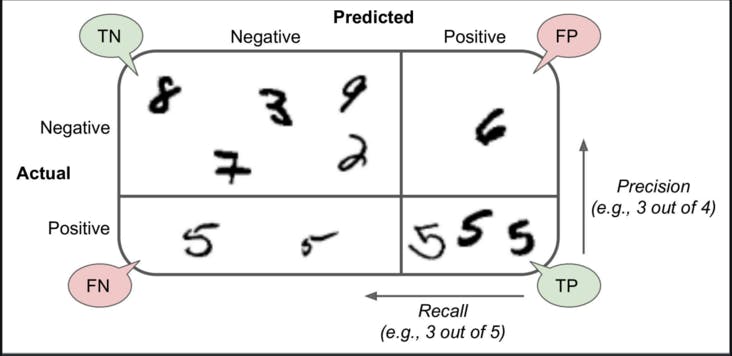
accuracyfocuses only on positive cases, not providing insights on how your model performs against negative cases (ie false negatives - FN). - BP - The confusion matrix is a much better way to evaluate the performance of a classifier:
sklearn.metrics.confusion_matrix. It gives you informations about true and false positives along with true and false negatives for each classification class. Illustration below:
- BP - It is often convenient to combine both metrics
precisionandrecallinto a single metric calledf1 score, (code ref.sklearn.metrics.f1_score)
- CS - A higher precision means your model is stricter with negative cases and can discard some positive instances, a higher recall means your model has more tolerance toward negative instances. Unfortunately, you can't have both at the same time, and the performance metric to favor depends on the problem you are solving. Otherwise, you want to tune your model parameters and training to reach an optimal precision/recall tradeoff.
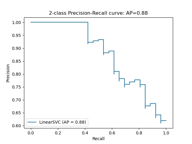
- BP - A good way to select the best precision/recall tradeoff is to plot the PR curve, representing the precision directly against recall using scikit-learn
decision_functionandsklearn.metrics.precision_recall_curve. Unlike theSGDClassifier, note thatRandomForestClassifierdoesn't have adecision_functionmethod, instead it has apredict_probamethod returning a row per instance and column per class, each containing the probability that the given instance belongs to the given class.
- BP - The ROC Curve (Receiver Operating Characteristic) is another common tool used with binary classifiers. Plotting recall (true positive rate) against the false positive rate (1 minus true negative rate) - code ref.
sklearn.metrics.roc_curve. It is also the entry point to visually represent the AUC (area under the curve) metric - code ref. sklearn.metrics.roc_auc_score - which is an effective way to compare classifiers since the perfect classifier will have a ROC AUC score of 1 v.s 0.5 for a random classifier. The closer to 1 the better. - BP - You should prefer the PR curve whenever the positive class is rare or when you care more about the false positives than the false negatives and the ROC curve otherwise.
- CS - Be mindful about the multiclass classification strategy, OneVsOne of OneVsAll as they come with change your model performance when scaling to larger dataset. Scikit-Learn has native support
- BP - When working on a multilabel classifications, meaning the ability for a classifier to provide multiple labels for one instance, (i.e Multiple people on the same picture), you might want to go with the
KNeighborsClassifier - BP - Use the test set only at the very end of your project, once you have a classifier that you are ready to launch.
In all, classification problems are somehow less straightforward than prediction problems when it comes to identify the metrics that will allow to spot the right model for your task. You want to select a good metric, pick the appropriate precision/recall tradeoff and compare classifiers to select the most performing one for your problem space.
Interestingly, you may want to check the classification Jupyter notebook to see these metrics and classifiers in action: Handsom ML - Chapter 3 solutions

